estimator

Modules

estimator module

class EstimationResult(result_x=None, component_id=None, component_attr=None, theta_mask=None, start_time=None, end_time=None, step_size=None, x0=None, lb=None, ub=None, iterations=None, nfev=None, final_objective=None, success=None, message=None)[source]

Bases: dict

A dictionary-like object containing parameter estimation results.

This class stores the results of parameter estimation including optimized parameters, component information, and metadata about the estimation process.

Parameters:

result_x (Optional[ndarray]) – Optimized parameter values.
component_id (Optional[List[str]]) – List of component IDs.
component_attr (Optional[List[str]]) – List of attribute names.
theta_mask (Optional[ndarray]) – Parameter mask.
start_time (Optional[List[datetime]]) – Training start times.
end_time (Optional[List[datetime]]) – Training end times.
step_size (Optional[List[int]]) – Training step sizes.
x0 (Optional[ndarray]) – Initial parameter values.
lb (Optional[ndarray]) – Lower bounds.
ub (Optional[ndarray]) – Upper bounds.
iterations (Optional[int]) – Number of iterations performed by the optimizer.
nfev (Optional[int]) – Number of function evaluations performed by the optimizer.
final_objective (Optional[float]) – Final objective function value achieved.
success (Optional[bool]) – Whether the optimization was successful.
message (Optional[str]) – Optimization result message.

Examples

>>> result = EstimationResult(
...     result_x=np.array([0.8, 0.9]),
...     component_id=["comp1", "comp2"],
...     component_attr=["efficiency", "efficiency"],
...     theta_mask=np.array([0, 1]),
...     start_time=[datetime.datetime(2024, 1, 1)],
...     end_time=[datetime.datetime(2024, 1, 2)],
...     step_size=[3600],
...     x0=np.array([0.7, 0.8]),
...     lb=np.array([0.5, 0.6]),
...     ub=np.array([1.0, 1.0]),
...     iterations=15,
...     nfev=45,
...     final_objective=0.00123,
...     success=True,
...     message="Optimization terminated successfully"
... )
>>> print(result["result_x"])
[0.8 0.9]
>>> print(result["iterations"])
15

copy()[source]: Create a shallow copy of the EstimationResult.

class Estimator(simulator)[source]

Bases: object

A class for parameter estimation in the twin4build framework.

This class provides methods for estimating model parameters using maximum likelihood estimation (MLE), with two different optimization approaches: Automatic Differentiation (AD) and Finite Difference (FD) methods.

Parameters:: simulator (Simulator) – The simulator instance for running simulations.

Mathematical Formulation:

The general parameter estimation problem is formulated as a maximum likelihood estimation:

\[\hat{\boldsymbol{\theta}} = \underset{\boldsymbol{\theta} \in \Theta}{\operatorname{argmax}} \; \mathcal{L}(\boldsymbol{\theta} | \boldsymbol{Y})\]

where:

\(\hat{\boldsymbol{\theta}}\) is the maximum likelihood estimate

\(\boldsymbol{\theta}\) is the parameter vector

\(\Theta \subseteq \mathbb{R}^{n_p}\) is the parameter space

\(\mathcal{L}(\boldsymbol{\theta} | \boldsymbol{Y})\) is the likelihood function

\(\boldsymbol{Y}\) are the observed measurements

Dimensions:

\(n_t\): Number of time steps in the simulation period
\(n_p\): Number of parameters to estimate
\(n_x\): Number of input variables (disturbances, setpoints, etc.)
\(n_y\): Number of output variables (measurements, performance metrics)

Model Structure:

The building model \(\mathcal{M}\) is represented as a directed graph where nodes are dynamic components and edges represent input/output connections.

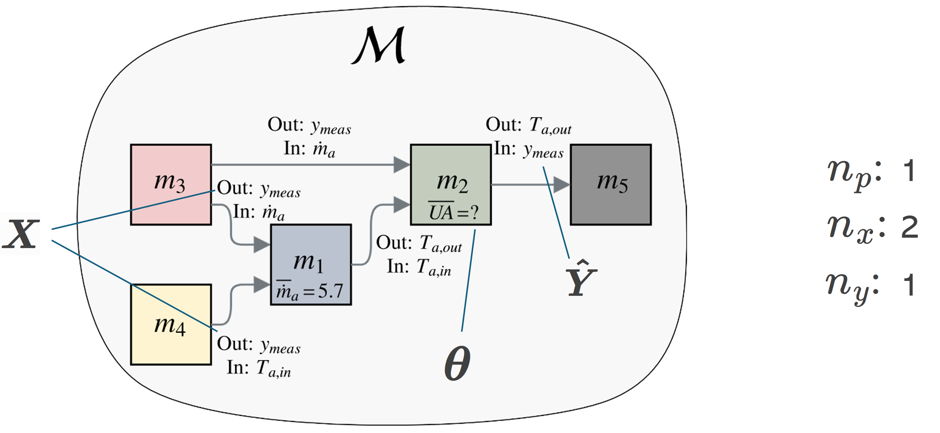
System overview showing components and their relationships

The model takes input variables \(\boldsymbol{X} \in \mathbb{R}^{n_x \times n_t}\) along with parameters \(\boldsymbol{\theta} \in \mathbb{R}^{n_p}\), and produces system outputs \(\boldsymbol{\hat{Y}} \in \mathbb{R}^{n_y \times n_t}\) with timesteps \(\boldsymbol{t} \in \mathbb{R}^{n_t}\):

\[\boldsymbol{\hat{Y}} = \mathcal{M}(\boldsymbol{X}, \boldsymbol{t}, \boldsymbol{\theta})\]

where \(\mathcal{M}\) represents the complete simulation model. See Simulator for detailed explanation of the simulation process.

Likelihood Function:

Using the Kennedy-O’Hagan (KOH) Bayesian model formulation, the relationship between observations \(\boldsymbol{Y}\), model response \(\boldsymbol{\hat{Y}}\), and measurement errors \(\boldsymbol{\epsilon}\) is:

\[\boldsymbol{Y}_j = \boldsymbol{\hat{Y}}_j + \boldsymbol{\epsilon}_j \quad \forall j \in \{1, \ldots, n_y\}\]

For normally distributed measurement errors, where \(\boldsymbol{\epsilon}_j \sim \mathcal{N}(\boldsymbol{0}, \boldsymbol{\Sigma}_j)\), the likelihood function becomes:

\[\mathcal{L}(\boldsymbol{\theta} | \boldsymbol{Y}) = \prod_{j=1}^{n_y} (2\pi)^{-n_t/2} \det(\boldsymbol{\Sigma}_j)^{-1/2} \exp\left(-\frac{1}{2}(\boldsymbol{Y}_j - \boldsymbol{\hat{Y}}_j)^T \boldsymbol{\Sigma}_j^{-1} (\boldsymbol{Y}_j - \boldsymbol{\hat{Y}}_j)\right)\]

where:

\(\boldsymbol{Y}_j \in \mathbb{R}^{n_t}\): Measured values for output \(j\) across all time steps

\(\boldsymbol{\hat{Y}}_j \in \mathbb{R}^{n_t}\): Model predictions for output \(j\) across all time steps

\(\boldsymbol{\Sigma}_j \in \mathbb{R}^{n_t \times n_t}\): Covariance matrix for output \(j\)

Taking the negative log-likelihood (for minimization) gives:

\[-\ln\mathcal{L}(\boldsymbol{\theta} | \boldsymbol{Y}) = \frac{n_t n_y}{2} \ln(2\pi) + \frac{1}{2} \sum_{j=1}^{n_y} \ln\det(\boldsymbol{\Sigma}_j) + \frac{1}{2} \sum_{j=1}^{n_y} (\boldsymbol{Y}_j - \boldsymbol{\hat{Y}}_j)^T \boldsymbol{\Sigma}_j^{-1} (\boldsymbol{Y}_j - \boldsymbol{\hat{Y}}_j)\]

With i.i.d. assumption and diagonal covariance matrices \(\boldsymbol{\Sigma}_j = \sigma_j^2 \boldsymbol{I}_{n_t}\), this simplifies to:

\[-\ln\mathcal{L}(\boldsymbol{\theta} | \boldsymbol{Y}) = \frac{n_t n_y}{2} \ln(2\pi) + \frac{n_t}{2} \sum_{j=1}^{n_y} \ln(\sigma_j^2) + \frac{1}{2} \sum_{j=1}^{n_y} \sum_{t=1}^{n_t} \left(\frac{Y_{j,t} - \hat{Y}_{j,t}}{\sigma_j}\right)^2\]

This is the form we use in twin4build for parameter estimation, meaning that we solve the following optimization problem:

\[\hat{\boldsymbol{\theta}} = \underset{\boldsymbol{\theta} \in \Theta}{\operatorname{argmin}} \; \sum_{j=1}^{n_y} \sum_{t=1}^{n_t} \left(\frac{Y_{j,t} - \hat{Y}_{j,t}}{\sigma_j}\right)^2\]

where the constant terms have been dropped since they do not affect the optimization.

Parameter Bounds:

For each parameter \(\theta_{i}\):

\[\theta_{i}^{lb} \leq \theta_{i} \leq \theta_{i}^{ub}\]

where:

\(\theta_{i}^{lb}\) is the lower bound

\(\theta_{i}^{ub}\) is the upper bound

See method docstrings for details on the specific optimization algorithms and implementation.

Examples

Basic usage with automatic differentiation (recommended):

>>> import twin4build as tb
>>> import datetime
>>> import pytz
>>>
>>> # Create model and simulator
>>> model = tb.SimulationModel(id="my_model")
>>> simulator = tb.Simulator(model)
>>> estimator = tb.Estimator(simulator)
>>>
>>> # Define parameters to estimate
>>> parameters = {
...     "private": {
...         "efficiency": {
...             "components": [component1, component2],
...             "x0": [0.8, 0.85],
...             "lb": [0.5, 0.6],
...             "ub": [1.0, 1.0]
...         }
...     },
...     "shared": {
...         "heatTransferCoefficient": {
...             "components": [[component1, component2]],
...             "x0": [[0.5]],
...             "lb": [[0.1]],
...             "ub": [[2.0]]
...         }
...     }
... }
>>>
>>> # Define measuring devices
>>> measurements = [measuring_device1, measuring_device2]
>>>
>>> # Set time period
>>> start = datetime.datetime(2024, 1, 1, tzinfo=pytz.UTC)
>>> end = datetime.datetime(2024, 1, 2, tzinfo=pytz.UTC)
>>> step = 3600
>>>
>>> # Run estimation with automatic differentiation (recommended)
>>> result = estimator.estimate(
...     parameters=parameters,
...     measurements=measurements,
...     start_time=start,
...     end_time=end,
...     step_size=step,
...     method=("scipy", "SLSQP", "ad")  # Preferred for most problems
... )

>>> # Alternative: Use L-BFGS-B with automatic differentiation
>>> result = estimator.estimate(
...     parameters=parameters,
...     measurements=measurements,
...     start_time=start,
...     end_time=end,
...     step_size=step,
...     method=("scipy", "L-BFGS-B", "ad")
... )

>>> # For non-PyTorch models: Use finite difference method
>>> result = estimator.estimate(
...     parameters=parameters,
...     measurements=measurements,
...     start_time=start,
...     end_time=end,
...     step_size=step,
...     method=("scipy", "trf", "fd"),
...     n_cores=4  # Required for FD mode
... )

>>> # Legacy string format (still supported)
>>> result = estimator.estimate(
...     parameters=parameters,
...     measurements=measurements,
...     start_time=start,
...     end_time=end,
...     step_size=step,
...     method="scipy"  # Defaults to SLSQP with AD
... )

estimate(start_time=None, end_time=None, step_size=None, parameters=None, measurements=None, n_warmup=60, method='scipy', n_cores=None, options=None, **kwargs)[source]

Perform parameter estimation using specified method and configuration.

This method sets up and executes the parameter estimation process, supporting both automatic differentiation (AD) and finite difference (FD) optimization methods.

Parameters:

start_time (Union[datetime, List[datetime], None]) – Start time(s) for estimation period(s). Can be a single datetime or list of datetimes for multiple periods.
end_time (Union[datetime, List[datetime], None]) – End time(s) for estimation period(s). Can be a single datetime or list of datetimes for multiple periods. Must be later than corresponding start_time.
step_size (Union[float, List[float], None]) – Step size(s) for simulation in seconds. Can be a single value or list of values for multiple periods.
parameters (Union[Dict[str, Dict], List[Tuple], None]) –
Parameter specifications in one of two formats:
New format (recommended): List of tuples where each tuple contains:
- component: The component object or list of component objects
- attr: Parameter attribute name (str)
- x0: Initial value (float)
- lb: Lower bound (float or None)
- ub: Upper bound (float or None)
- parameter_type: “private” or “shared” (optional, defaults to “private”)
Parameter types:
- ”private”: Each component gets its own independent parameter
- ”shared”: All components in the list share the same parameter value
Examples

```python # Private parameters (default) parameters = [

(space, “thermal.C_air”, 2e+6, 1e+6, 1e+7), # implicit “private” (space, “thermal.C_wall”, 2e+6, 1e+6, 1e+7, “private”), # explicit ([controller1, controller2], “kp”, 0.001, 1e-5, 1, “private”), # separate kp for each

]

# Shared parameters parameters = [

([space1, space2], “thermal.C_air”, 2e+6, 1e+6, 1e+7, “shared”), # same C_air value ([controller1, controller2], “kp”, 0.001, 1e-5, 1, “shared”), # same kp value
Legacy format (deprecated): Dictionary containing parameter specifications:
- ”private”: Parameters unique to each component
- ”shared”: Parameters shared across components
Each parameter entry contains:
- ”components”: List of components or single component
- ”x0”: List of initial values or single initial value
- ”lb”: List of lower bounds or single lower bound
- ”ub”: List of upper bounds or single upper bound
measurements (Optional[List[System]]) – List of measuring devices used for estimation. Each device should have an “input” attribute with a “measuredValue” that contains historical data.
n_warmup (int) – Number of simulation steps used to initialize the model. These are not included in the likelihood calculation.
method (Union[str, Tuple[str, str, str]]) –
Estimation method specification. Can be specified in two formats:

1. String format (legacy): - “scipy”: Uses default SLSQP optimizer with automatic differentiation - Other valid strings: Any optimizer name that matches the supported algorithms

(e.g., “L-BFGS-B”, “TNC”, “SLSQP”, “trust-constr”, “trf”, “dogbox”)

2. Tuple format (recommended): - (library, optimizer, mode) where:
- library: “scipy” (currently the only supported library)
- optimizer: The specific optimization algorithm
- mode: “ad” (automatic differentiation) or “fd” (finite difference)
Supported optimizers by mode:

Automatic Differentiation (AD) mode: - “SLSQP”: Sequential Least Squares Programming (preferred for most problems) - “L-BFGS-B”: Limited-memory BFGS with bounds - “TNC”: Truncated Newton algorithm with bounds - “trust-constr”: Trust-region constrained optimization - “trf”: Trust Region Reflective (for least-squares problems) - “dogbox”: Dogleg algorithm (for least-squares problems)

Finite Difference (FD) mode: - “trf”: Trust Region Reflective (for least-squares problems) - “dogbox”: Dogleg algorithm (for least-squares problems)

Mode selection guidelines: - “ad”: Use when all components are torch.nn.Module (preferred, faster) - “fd”: Use for non-PyTorch models or mixed model types (requires n_cores)

Examples: - (“scipy”, “SLSQP”, “ad”): Preferred for most PyTorch models - (“scipy”, “trf”, “fd”): For non-PyTorch models with least-squares formulation - “scipy”: Legacy format, defaults to (“scipy”, “SLSQP”, “ad”)
n_cores (Optional[int]) –
Number of CPU cores to use for parallel computation. Required when using finite difference (FD) mode for Jacobian computation. Not used in automatic differentiation (AD) mode.
- For FD mode: Must be specified (typically 2-8 cores depending on system)
- For AD mode: Ignored (not needed for automatic differentiation)
- Default: None (will raise error if FD mode is used without specifying)
options (Optional[Dict]) –
Additional options for the chosen optimization method:
For scipy optimizers:
- ”ftol”: Function tolerance (default: 1e-8)
- ”xtol”: Parameter tolerance (default: 1e-8)
- ”gtol”: Gradient tolerance (default: 1e-8)
- ”maxiter”: Maximum iterations
- ”verbose”: Verbosity level

Returns:

Object containing the estimation results including optimized parameters, component information, and metadata.

Return type:

EstimationResult

Raises:

AssertionError – If method specification is invalid or input parameters are inconsistent.
ValueError – If method format is incorrect or unsupported.
FMICallException – If simulation fails during parameter evaluation.

Notes

The method automatically handles parameter normalization and bounds checking.
For AD mode, all components must be torch.nn.Module instances.
For FD mode, n_cores must be specified for parallel Jacobian computation.
Results are automatically saved to disk in the model’s estimation_results directory.
Multiple time periods are supported by providing lists for start_time, end_time, and step_size.

Examples

>>> # New list format (recommended)
>>> parameters = [
...     (space, "thermal.C_air", 2e+6, 1e+6, 1e+7),  # private (default)
...     ([space1, space2], "thermal.C_wall", 2e+6, 1e+6, 1e+7, "shared"),  # shared
...     (heating_controller, "kp", 0.001, 1e-5, 1, "private"),  # explicit private
... ]
>>> result = estimator.estimate(
...     parameters=parameters,
...     measurements=devices,
...     start_time=start,
...     end_time=end,
...     step_size=3600,
...     method=("scipy", "SLSQP", "ad")
... )

>>> # Legacy dict format (deprecated but still supported)
>>> parameters = {
...     "private": {
...         "efficiency": {
...             "components": [component1, component2],
...             "x0": [0.8, 0.85],
...             "lb": [0.5, 0.6],
...             "ub": [1.0, 1.0]
...         }
...     }
... }
>>> result = estimator.estimate(
...     parameters=parameters,
...     measurements=devices,
...     start_time=start,
...     end_time=end,
...     step_size=3600
... )